
Orbital Equations Overview
Orbital Equations are the programs used to define Orbital Fractals in the Fractal Science Kit fractal generator. Before you begin, please read the Orbital Fractal Overview.
See also:
- Orbital Fractal Overview
- Base Equations
- Properties Window
- Program Editors
- Fractal Programs
- Program Instructions
- Programming Language
Each program is composed of a set of properties and instructions.
Comments
Always remember to click the Toggle Code View toolbar button at the top of the Program Editor and read the comments given in the comment section of the program's instructions. The comment section contains usage instructions, hints, notes, documentation, and other important information that will help you understand how best to use the program. Once you are done reading the comments, click the Toggle Code View toolbar button again to view the program's properties.
Properties
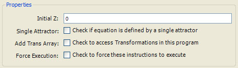
The following properties are supported:
-
Initial Z is a numeric textbox used to enter a complex value for the Initial Z. If the initial z value is dependent on selected properties set by the user, you will need to initialize z in the initialize section of the program instructions and the Initial Z property can be ignored.
-
Single Attractor is a checkbox that can be checked to indicate the equation is defined by a single attractor. This is frequently the case with strange attractors. This affects how the attractorIndex variable is interpreted. See the discussion below for details.
-
Add Trans Array is a checkbox that can be checked to add a Transformation Array editor as one of the program's properties pages. Users can add 1 or more transformations to the editor and your program can access the transformations using the Transformation Functions.
-
Force Execution is a checkbox that can be checked to force execution of the instructions. If Force Execution is unchecked, the instructions will execute only if required based on what changes were made to the fractal's properties since the last time the instructions ran. This is checked for those programs that search for interesting parameter settings based on user defined criteria since these programs need to execute even if no changes are made to their properties.
Instructions
The remainder of this page can be ignored if you are not a programmer.
At the bottom of the window is an editor pane named Instructions. The editor pane is a simple text editor to view/edit your Program Instructions. See Editing Text for details.
The instructions are divided into sections. Within each section are statements that conform to the Programming Language syntax.
In addition to the Standard Sections, Orbital Equations support 2 other sections:
initialize:
iterate:
The initialize section is executed once, just prior to beginning the orbit. Instructions that need to execute at the beginning of the iteration should be placed here. The iterate section is executed once per iteration and is the primary section of the Orbital equation.
Example:
comment:
This program generates a Sierpinski Triangle.
This fractal was described by Waclaw Sierpinski
in 1915!
The fractal exterior is an equilateral triangle.
The options Center and Radius control the size
and position of the triangle's circumcircle.
The Angle option is used to rotate the triangle
counterclockwise.
For details see:
http://mathworld.wolfram.com/SierpinskiSieve.html
http://en.wikipedia.org/wiki/Sierpinski_triangle
global:
const Complex point[3]
Geometry.GeneratePointsOnCircle( \
point[], 3, Center, Radius, DegreeToRadian(Angle) \
)
iterate:
attractorIndex = Random.Integer(3)
z = Geometry.MidPoint(z, point[attractorIndex])
properties:
option Center {
type = Complex
caption = "Center"
details = "Center of equilateral triangle"
default = 0
}
option Radius {
type = Float
caption = "Radius"
details = "Radius of triangle circumcircle"
default = 1
range = (0,)
}
option Angle {
type = Float
caption = "Angle"
details = "Angle of rotation"
default = 0
range = [-360,360]
}
These instructions can be used to produce the Sierpinski Triangle. The global section initializes the point[] array with the vertices of an equilateral triangle inscribed in the circle given by the properties Center and Radius, rotated by Angle degrees. On each iteration, one of the vertices is selected at random as the attractor, and the point z is shifted to the midpoint of the segment connecting the current value of z and the selected vertex.
The variables z and attractorIndex are used to return the results computed by the program. z is the value computed for the next orbit point. attractorIndex is an index between 0 and 255 that is mapped to the sample point's AttractorIndex field which can be used by the controller to assign a color to the sample. Typically, as in this example, attractorIndex is an index identifying which attractor influenced z on this iteration.
Some of the Orbital Equations are driven off data contained in files. For example, the IFS File Processor reads an IFS definition from a file. The file must conform to the specification defined by Fractint for its IFS files (2D only). These files contain a set of IFS definitions, each in the form:
<Name> {
<A> <B> <C> <D> <E> <F> <Probability>
...
}
<Name> is the name of the IFS. <A>, <B>, <C>, <D>, <E>, and <F> are the fields associated with an affine transformation, and <Probability> is the associated probability. The set of affine transformations and their associated probabilities define the IFS. Multiple definitions can be placed in a file.
Example IFS file with a single IFS definition:
fern {
0.85 0.04 -0.04 0.85 0.0 1.6 0.85
0.2 -0.26 0.23 0.22 0.0 1.6
0.07
-0.15 0.28 0.26 0.24 0.0 0.44 0.07
0.0 0.0 0.0 0.16 0.0
0.0 0.01
}
The IFS File Processor program reads files of this type using a DataFile Statement. The dataFile statement defines a file format and includes controls on the Properties Page to select a dataset within a file. The selected dataset is loaded into a 2-dimensional array and is available to the program instructions.
IFS File Processor instructions:
global:
count = Array.Dim1(DataTable[,])
const Complex indexLUT[10000]
const Affine s[count]
Complex w[count]
'
' Initialize Affine array s[] and weight array w[].
'
for (i = 0, i < count, i += 1) {
offset = Array.Offset(DataTable[,], i, 0)
Array.Copy(DataTable[,], offset, s[], i, 6)
w[i] = DataTable[i, 6]
}
Affine.ScaleDimension(s[], count, Factor)
Math.GenerateIndexLookupTable(w[], count, indexLUT[])
iterate:
attractorIndex = Math.GenerateIndex(indexLUT[])
z = Affine.TransformPoint(s[attractorIndex], z)
properties:
option Factor {
type = Float
caption = "Affine Factor"
details = "Use factor < 1 to sharpen, factor > 1 to blur"
default = 1
}
dataFile DataTable {
path = "Examples.ifs"
type = "IFS"
suffix = "ifs"
columns = 7
}
The file format is defined using the statement:
dataFile DataTable {
path = "Examples.ifs"
type = "IFS"
suffix = "ifs"
columns = 7
}
This statement reads files that conform to the Fractint syntax and allows the user to select one of the datasets contained in the file using a control on the program's Properties Page. The selected dataset is loaded into the 2-dimensional array named DataTable[,] for use in the program. Our program converts the 2-dimansional array of Complex values into a 1-dimensional array of Affine objects named s[] and a 1-dimensional array of weights w[] using the following statements:
for (i = 0, i < count, i += 1) {
offset = Array.Offset(DataTable[,], i, 0)
Array.Copy(DataTable[,], offset, s[], i, 6)
w[i] = DataTable[i, 6]
}
The weights are used to generate an array of index values in a look-up table (indexLUT[]) that we will use to generate random values based on the weights. By using the index look-up table as illustrated here, you can speed up the iterate section of your program which is the most expensive portion of the Orbital Equation.
Finally, the iterate section simply generates a random index into the array of Affine objects (s[]) and transforms z using the selected Affine transformation.
iterate:
attractorIndex = Math.GenerateIndex(indexLUT[])
z = Affine.TransformPoint(s[attractorIndex], z)
The variables z and attractorIndex return the results computed by the program. attractorIndex is an index identifying which attractor influenced z on this iteration. z is the value computed for the next orbit point using the selected Affine transformation (s[attractorIndex]).
The FSK.OverrideValue method can be used to override selected parameter settings. See FSK Functions for details.
Built-in Variables
Several built-in variables are available to your instructions:
- z
- attractorIndex
- zprev1
- zprev2
The variables z and attractorIndex are used to return the results computed by the program. All of the remaining variables are read-only.
z is the value computed for the next orbit point. attractorIndex is an index between 0 and 255 that is mapped to the sample point's AttractorIndexRaw field which can be used by the controller to assign a color to the sample. Typically, (as in the above examples) attractorIndex is an index identifying which attractor influenced z on this iteration.
zprev1 and zprev2 are the previous 2 values of z in the orbit. In addition to zprev1 and zprev2, you can access the orbit points available in the orbit point buffer using the Orbit Functions.
Sometimes, the Orbital fractal is defined using a single attractor. In these cases, you should check the Single Attractor checkbox in the Properties section and set the attractorIndex to a number (a float) used to color the sample. Typically, you can use the distance from the origin to the input point z, as in the following example.
Example:
iterate:
attractorIndex = Abs(z)
z = Complex( \
Sin(A*z.y) + C*Cos(A*z.x), \
Sin(B*z.x) + D*Cos(B*z.y) \
)
properties:
option A {
type = Float
caption = "A"
default = 0
range = [-3,3]
}
option B {
type = Float
caption = "B"
default = 0
range = [-3,3]
}
option C {
type = Float
caption = "C"
default = 0
range = [-3,3]
}
option D {
type = Float
caption = "D"
default = 0
range = [-3,3]
}
Setting the attractorIndex to Abs(z) before we update z, colors the sample based on the location of the previous orbit point. When you check the Single Attractor checkbox, the Fractal Science Kit will normalize the value you set attractorIndex to and save the value as an integer between 0 and 255 that is mapped to the sample point's AttractorIndexRaw field.