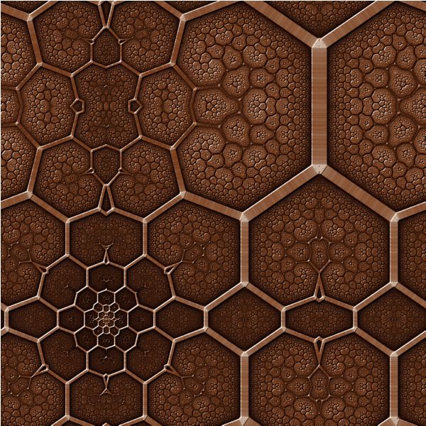
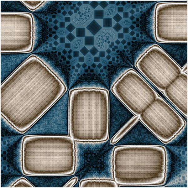
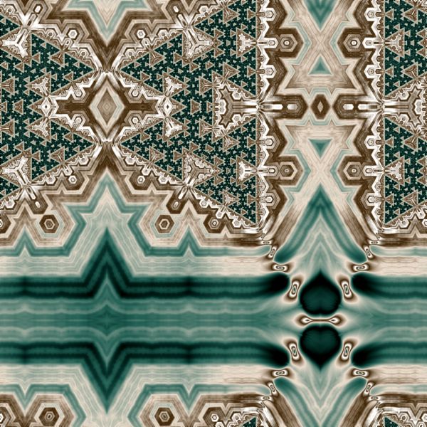
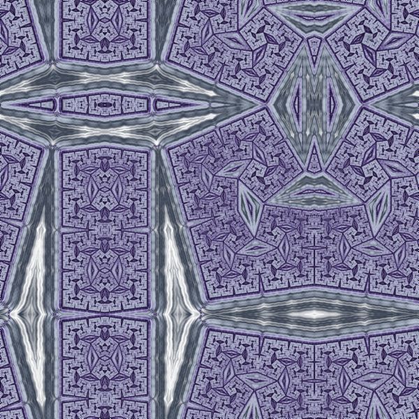
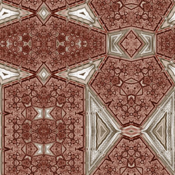
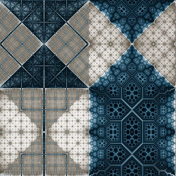
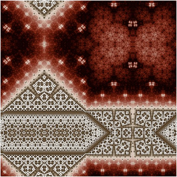
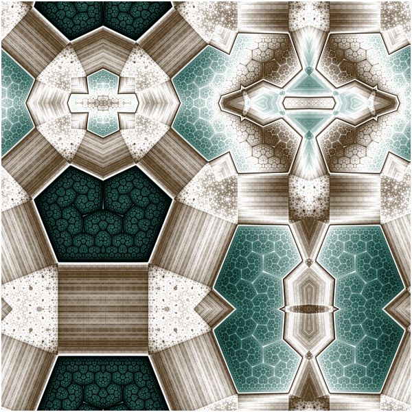
Julia Pattern Map (page 1)

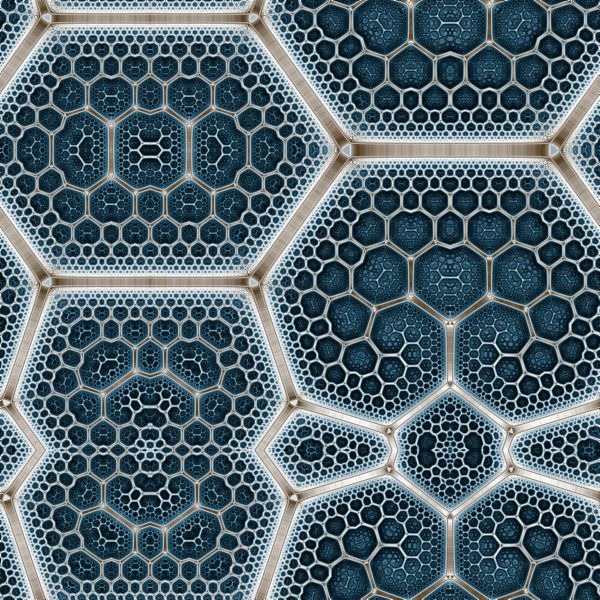
Home • Gallery • Tutorials • Download • Purchase • Site Map

Julia Pattern Map Examples

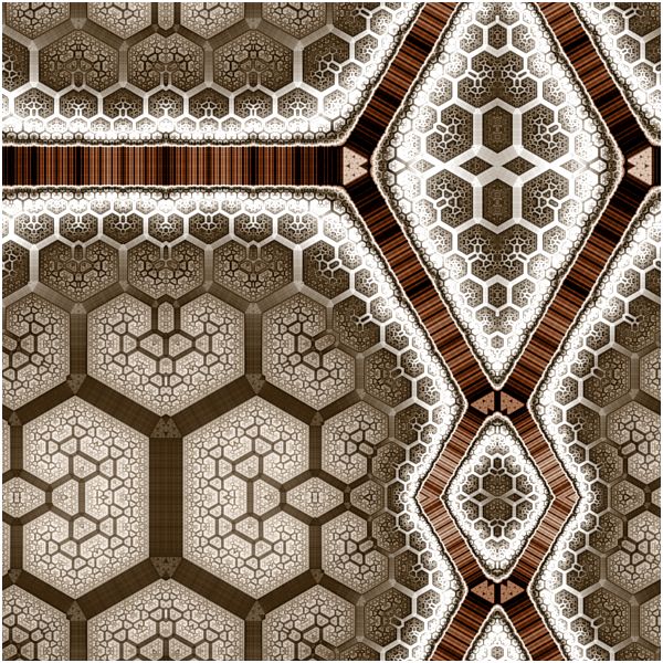
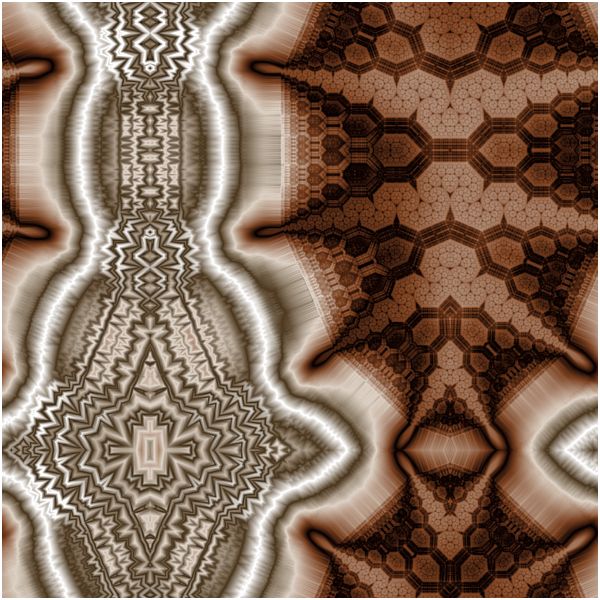
Alien Hive Julia Pattern Map 01	Pillars of Steel Julia Pattern Map 04	Fluid Dynamics Julia Pattern Map 05
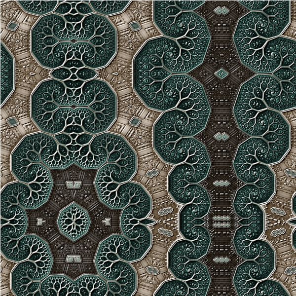
Titanium Web Julia Pattern Map 06	Living Blocks Julia Pattern Map 07	Woodland Garden Julia Pattern Map 09
Contrasting Values Julia Pattern Map 10	Cognitive Architecture Julia Pattern Map 11	Synaptic Pathways Julia Pattern Map 12
Cellular Network Julia Pattern Map 13	Charging Station Julia Pattern Map 14	Fuel Injection Julia Pattern Map 15
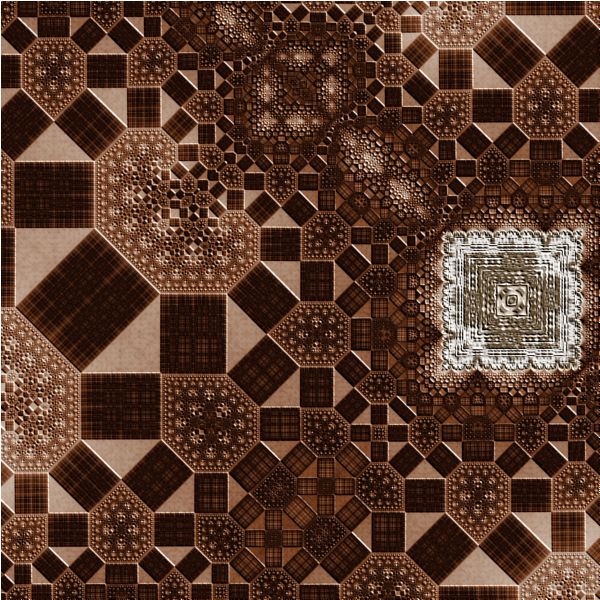
Binding Energy Julia Pattern Map 17	Koch's Grove Julia Pattern Map 20	Block Factory Julia Pattern Map 21
Cracked Stone I Julia Pattern Map 22	Cracked Stone II Julia Pattern Map 23	Patchwork Design Julia Pattern Map 24
Polished Wood Inlay Julia Pattern Map 25	Invasion Force Julia Pattern Map 26	Emerald Sky Julia Pattern Map 27

The Julia Pattern Map examples display a Julia Fractal based on the Fractal Equation Julia Pattern Map.

The Julia Pattern Map equation was inspired by work done by Pablo Roman Andrioli (Kali) described in the Fractal Forums post Very simple formula for fractal patterns.

Note the following:

Example	Alternate Value
Julia Pattern Map 01	Exponential Smoothing (Delta)
Julia Pattern Map 04	Exponential Smoothing (Delta)
Julia Pattern Map 05	Exponential Smoothing (Delta)
Julia Pattern Map 06	Exponential Smoothing (Delta)
Julia Pattern Map 07	Exponential Smoothing (Delta)
Julia Pattern Map 09	Exponential Smoothing (Delta)
Julia Pattern Map 10	Exponential Smoothing (Delta)
Julia Pattern Map 11	Average Angle
Julia Pattern Map 12	Average Angle
Julia Pattern Map 13	Average Angle
Julia Pattern Map 14	Average Angle
Julia Pattern Map 15	Exponential Smoothing (Optimized)
Julia Pattern Map 17	Exponential Smoothing (Delta)
Julia Pattern Map 20	Exponential Smoothing (Delta)
Julia Pattern Map 21	Exponential Smoothing (Delta)
Julia Pattern Map 22	Exponential Smoothing (Delta)
Julia Pattern Map 23	Exponential Smoothing (Delta)
Julia Pattern Map 24	Exponential Smoothing (Delta)
Julia Pattern Map 25	Exponential Smoothing (Delta)
Julia Pattern Map 26	Average Angle
Julia Pattern Map 27	Average Angle

The Alternate Value setting is used to generate data that is used by the Color Controller to generate the image.

Overview

These Julia Fractals are based on 3 different built-in programs working together to generate the final image; the Julia Pattern Map Fractal Equation, the Alternate Value (given in the table above) and the Gradient Map - Value Color Controller. The Julia Pattern Map Fractal Equation is the heart of the fractal. For each pixel of the image, the Julia Pattern Map generates a fractal orbit; i.e., a set of points on the complex plane generated as we apply the equation over and over again. These points are passed to the Alternate Value which processes them and generates a data value used by the Gradient Map - Value Color Controller to color the pixel. So, the choices you make when setting up these 3 programs are what determines what your fractal will look like.

I found each of these Julia Fractals using the example Julia Pattern Map 00 (not pictured above). The example Julia Pattern Map 00 is a Mandelbrot Fractal with Anti-Aliasing turned off to increase performance as you explore, as recommended in the Fractal Science Kit Examples Overview. The following describes how to use this example to find your own fractals similar to the examples found here.

The general process you will use, is to open Julia Pattern Map 00, change a few properties associated with the Julia Pattern Map Fractal Equation, optionally change the Alternate Value and/or its properties, and display the resulting Mandelbrot Fractal. Next, use the Preview Julia command to explore the Mandelbrot's many different Julia Fractals. Once you find an interesting Julia fractal, you can use the Gradient Map - Value Color Controller to map the data generated by the selected Alternate Value, to a color gradient to generate the image. This process is described in detail in the following sections.

Change the Julia Pattern Map Properties

First, open Julia Pattern Map 00 and navigate to the Julia Pattern Map equation's properties page:

General
    Mandelbrot / Julia / Newton
        Fractal Equation: Julia Pattern Map
            Properties

This page controls the orbit generation that defines the fractal image.

Max Dwell controls the number of points in the orbit. The fractal image is very sensitive to changes in this value. Large values (i.e., greater than 50) tend to turn the image into a static mess so I recommend you leave the value at 16 initially. Once you find a Julia Fractal you like using the process described below, you can return to this page and increase this value a little (e.g., between 16 and 32) to add complexity to the image. You will need to try several values to find the best results. More on this later.

Pattern Map, Overlay, Radius, and C Map, define the equation. Pattern Map controls which of the 22 predefined patterns to use. Overlay applies a second version of the pattern, rotated by Overlay*45 degrees. An Overlay of 0 turns off the overlay and is the default setting. Radius controls the radius of the circle of inversion used to keep the orbit constrained inside the circle. A Radius value between 3 and 24 is recommended. Finally, C Map controls the method used to combine the orbit value z (modified by Pattern Map, Overlay, and Radius) with the complex value c (the Julia Constant when dealing with Julia Fractals). Most of the examples use the default setting for Overlay and Radius, and use Pattern Map and C Map to alter the fractal. If you don't understand any of this, don't worry! Just know that you can change these value to whatever you like and you will get a different fractal result. In fact, understanding what these values do, does not help you in any way with respect to knowing what the resulting fractal will look like based on your choices!

The remaining options inject a kaleidoscope transformation into the equation. Note that currently, none of the examples use this feature, but some may in the future when I get around to playing with these options myself! Feel free to experiment.

There are also 3 additional properties pages associated with the Julia Pattern Map equation; i.e., Pre-Map Transformation, Post-Map Transformation, and Final Transformation. Each of these defines an affine transformation applied at different stages of the equation's processing. The following gives the processing details:

Apply Pre-Map Transformation
Apply Pattern Map
Apply Overlay
Apply Post-Map Transformation
Apply Circle Inversion if the value is outside circle of the given Radius
Apply C Map
Apply Final Transformation

Most of the examples do not use these transformations, but a few use the Post-Map Transformation to alter the value slightly prior to passing it to the C Map. Examine the specific examples for details. Each affine transformation is defined as a set of simple transformations (translations, rotations, reflections), that are applied in the given order, to define the affine transformation. You can experiment with these if you like but it is an advanced feature that can be ignored for now.

So, in summary, I recommend that you change 0 or more of the options Pattern Map, Overlay, Radius, and C Map and proceed to the next section.

Change the Alternate Value

The Alternate Value is used to process the orbit generated by the Julia Pattern Map equation, and generate a value that will be used by the Gradient Map - Value Color Controller to color the pixel. As you can see from the table at the top of this page, the examples use a variety of different Alternate Values. The Julia Pattern Map 00 example is configured to use the Exponential Smoothing (Delta) Alternate Value but you can experiment with any of the other Alternate Values as well.

Navigate to the Alternate Mapping 1 page:

General
Mandelbrot / Julia / Newton
Alternate Mapping 1: Instructions

You can set the Alternate Mapping by changing the Type property. The other values on this page, in the Alternate 1 Value Normalization section, should be left as they are for now. They control the data normalization and I will discuss them later.

Type, which selects the type of data that you wish to collect, is one of the following values:

Depending on your choice, a different set of dependent pages is shown in the page hierarchy.

Any of the settings are good when used with the Julia Pattern Map equation except <None>, which disables the orbit data processing, and the Orbit Trap Statistic, which is not useful in this context. The only 2 settings used by the examples at this time are Instructions (used by all but a handful of the examples) and Orbit Trap Minimum but the others also provide good results with this type of fractal.

If you set the mapping to Instructions, a Program Editor for an Alternate Value is displayed in the page hierarchy under the Alternate Mapping page. This setting is the most flexible since it provides you with full control over the data collection processing. The remaining settings are less flexible but highly optimized. Many of these settings provide additional pages in the page hierarchy that control different aspects of the data collection.

You should stick with Instructions for now (which is what the Julia Pattern Map 00 example is configured to use), and later you can try out some of the other settings.

Navigate to the Exponential Smoothing (Delta) page:

General
    Mandelbrot / Julia / Newton
        Alternate Mapping 1: Instructions
            Exponential Smoothing (Delta)

This is a Program Editor for an Alternate Value. The Julia Pattern Map 00 example is set to the Exponential Smoothing (Delta) Alternate Value which is used by many of the examples.

Select the Properties page to view the options associated with the Exponential Smoothing (Delta) Alternate Value:

General
    Mandelbrot / Julia / Newton
        Alternate Mapping 1: Instructions
            Exponential Smoothing (Delta)
                Properties

The Processing Options section controls how the data values are generated by the program. The Value Expression controls the expression used by the program. The Distance Metric and Power are applied to the expression value to get the value to accumulate over the orbit.

The Orbit Generation section controls which orbit points are used when computing the value. By changing these value, you can affect the resulting value passed to the color controller. For example, setting Mod Dwell to 2 would use only the odd orbit points; i.e., those with dwell values 1, 3, 5, etc. If you also set Min Dwell to 2, you would use only the even orbit points; i.e., those with dwell values 2, 4, 6, etc.

Changes to any of these values, will change the values passed to the color controller and therefore change how the image will look. Experimentation is the key.

In addition to Exponential Smoothing (Delta), several of the other Alternate Value programs are used by the examples as shown in the table at the top of this page. To use a different program, return to the Exponential Smoothing (Delta) page:

General
    Mandelbrot / Julia / Newton
        Alternate Mapping 1: Instructions
            Exponential Smoothing (Delta)

Change the Based On property to one of the following values:

Exponential Smoothing (Optimized)
Exponential Smoothing (Delta)
Exponential Smoothing (Triangle Metric Value)
Blended Value
Statistics
Minimum Value/Delta
Minimum Shape
Average Angle

These are the values that work best with the Julia Pattern Map equation. For each Alternate Value, visit the Properties page found under the program in the page hierarchy, to view the program's properties. Be sure to experiment with changes to the properties.

After you select 1 of the Alternate Values and have made any changes (optional) to the properties on the Properties page, you are ready to generate the Mandelbrot fractal which you will use to find the Julia fractals.

Generate the Mandelbrot Fractal

To generate the Mandelbrot fractal image, execute the Display Fractal command on the Tools menu. The resulting fractal will not be much to look at, but it is your key to finding new Julia Fractals similar to the examples above. In fact, every one of the examples was found using a Mandelbrot similar yours, using the procedure described below.

Generating Julia Fractals

When you generate a Julia Fractal, you need to select a Julia Constant. The choice of the Julia Constant in large part controls the character of the resulting Julia fractal. Surprisingly, the Mandelbrot fractal for the same fractal formula provides the best interface for choosing the Julia Constant. The Mandelbrot fractal can be used as a map for choosing the Julia Constant. To this end, the Fractal Science Kit allows you to activate the Preview Julia setting so that clicking on the Mandelbrot fractal will produce a Julia fractal in a small window called the Preview Window. Clicking on the image displayed in the Preview Window causes the Julia fractal to be displayed in a full size window for further exploration.

Select the Preview Julia item found on the Tools menu. This changes the cursor to a cross and places the Fractal Window into a state where clicking on the Mandelbrot fractal generates a Julia fractal preview in the Preview Window. The point on the Mandelbrot fractal where you click is used as the Julia Constant for the preview. There is a single Preview Window shared by all windows and each click on the Mandelbrot image generates a new Julia fractal preview, replacing any image currently in the Preview Window. If you wish to cancel the operation, simply select the Preview Julia menu item or toolbar button again. While you are in this state, the Preview Julia menu item has a check next to it and the Preview Julia toolbar button is depressed. See Exploring Julia Fractals for details.

As you click on different location on the Mandelbrot image, you will see the resulting Julia fractal in the Preview Window. You should experiment by clicking in various spots on the image, looking for interesting Julia fractals. You will find that small changes in where you click on the Mandelbrot will result in very large changes in how the associated Julia will look. I frequently zoom into the Mandelbrot, when I am trying to find just the right place to click to get the best result.

Once you have an image in the Preview Window that you like, you should click on it to generate a full size window that displays the Julia fractal.

Mapping the Data to Color

Once you have a full size window that contains a Julia fractal that looks interesting, you are ready to work with the data normalization settings and the color controller to adjust the color mapping used to produce your fractal. Frequently, you can turn an unattractive image into a beauty simply by adjusting the color mapping!

It is understood that all the remaining properties changes described below are to the properties associated with the Julia fractal, not the Mandelbrot we have been changing thus far. So you need to close the Properties Window for the Mandelbrot fractal and open a new Properties Window for the Julia fractal by clicking on the Properties Window item on the View menu for the Fractal Window that contains the Julia fractal.

There are 2 places that allow you to control the mapping of data to colors; the data normalization settings associated with the Alternate Value, and the Gradient Map - Value color controller properties. Whether you use one or both of these is up to you. None of these properties change the data you have generated, so any changes you make will not require the data to be regenerated and therefore the update will be relatively fast. You should experiment with both sets of properties so that you get a feeling of what they do, and then when you are looking for just the right coloring for one of your fractals, you will know where to go.

Working With Data Normalization

Navigate to the Alternate Mapping 1 page:

General
Mandelbrot / Julia / Newton
Alternate Mapping 1: Instructions

Important: Do not change the Type property.

The other values on this page, in the Alternate 1 Value Normalization section, control the data normalization. The properties on this page are explained on the Data Normalization page of the documentation. In 99% of the cases, the only properties you should change are Transfer Function and Power. See Transfer Function for details.

After you make changes to one or both of these properties, you should execute the Display Fractal command on the Tools menu of the Fractal Window for the Julia fractal to view the results. Experiment with the different choices until you get something you like.

Working With the Color Controller

Select the Gradient Map - Value properties page:

General
    Mandelbrot / Julia / Newton
        Classic
            Controllers
                Gradient Map - Value

This page is a Program Editor for the Classic Controller Gradient Map - Value.

The 2 sets of properties I frequently change on this page are those in the sections called Color Space Adjustment and Color Adjustment. See Classic Controller for a description of these properties in the sections of the same name.

I should point out here that a few of the examples use a custom gradient to take full control of how the data is mapped to color. You can do this too by editing one of the gradients found on this page or by adding one of your own gradients to the controller's list of available gradients. See Gradient List Control and Gradient Editor for details. See Gradient Browser for loading your existing gradients into the Fractal Science Kit.

The properties specific to the Gradient Map - Value controller are found on the Properties page:

General
    Mandelbrot / Julia / Newton
        Classic
            Controllers
                Gradient Map - Value
                    Properties

Color Scheme is used to control which color gradient to use.

Value is the data value used to color the image and is set to Alternate 1 Value. This is the value produced by Alternate Mapping 1 and normally, should not be changed. In rare cases, the Alternate Value sets both Alternate 1 Value and Alternate 1 Angle (e.g., Statistics, Minimum Shape), and in those cases you could set Value to one of the following:

Alternate 1 Angle
Alternate 1 Angle (Bounce)
Alternate 1 Angle (Cos)

However, these Alternate Values (i.e., Statistics, Minimum Shape) also have a property called As Value which can be used to return the angle as Alternate 1 Value to allow for more control over data normalization and is recommended for those cases where you want to use the angle for coloring. In short, you rarely need to change the Value property.

Power, Factor, and Offset, control how the data is mapped to the gradient given by Color Scheme. Power is applied first, then Factor, and finally, Offset. These are described below.

The normalized data ranges from 0 to 1 as do the gradient values. We start with the normalized value between 0 and 1 and apply the Power, Factor, and Offset, and then find the corresponding gradient value which we use to color the pixel. If the value is outside the range 0 to 1, we wrap the value into that range prior to mapping to the gradient.

Power is used as an exponent to alter the value (i.e., the value is raised to the given Power), Factor is used to scale the value, and Offset is used to shift the value. Mathematically, we have:

Value = Value^Power
Value = Value*Factor
Value = Value+Offset

or more concisely:

Value = Offset + Factor*Value^Power

Power controls how quickly the data moves through the gradient. If Power is set to a value between 0 and 1, the smaller data values consume most of the gradient. If Power is greater than 1, the larger data values consume most of the gradient. Normally, Power is between 0.5 and 2.

Factor changes the range and direction of the data. Normally the data range is 0 to 1. By using a Factor of 0.5, you would change the range of the data to 0 to 0.5, effectively eliminating half the gradient. Using a Factor of 2, you would map the data over the gradient twice. Using a Factor of -1 would reverse the direction of movement through the gradient, moving from right to left through the gradient rather that from left to right as is normal.

Offset controls where data value 0 falls within the gradient. An Offset of 0.5, for example, would map data value 0 into the middle of the gradient (0.5 is the middle of the gradient). Therefore data values in the range 0 to 0.5 would map to the upper half of the gradient (0.5 to 1), and data values in the range 0.5 to 1 would wrap around and map to the lower half of the gradient (0 to 0.5).

Adjusting Complexity

Once you have an image you like, you can try to adjust the complexity to see what looks best.

Select the Julia Pattern Map equation's properties page:

General
    Mandelbrot / Julia / Newton
        Fractal Equation: Julia Pattern Map
            Properties

Adjust Max Dwell to increase/decrease complexity to see what looks best.

Remember, Max Dwell controls the number of points in the orbit. The fractal image is very sensitive to changes in this value. Increase this value a little (e.g., between 16 and 32) to add complexity to the image. You will need to try several values to find the best results. Small changes work best.

Transformations

You can apply a transformation to your fractal as described below. Note that only 1 of the examples use a transformation.

To apply a transformation to the fractal, select the Identity transformation's page:

General
    Mandelbrot / Julia / Newton
        Transformation
            Identity

Change the Based On property to select a transformation and then open the transformation's properties page (found under the transformation in the page hierarchy), and play with the transformation's properties. See Transformation Support for details.

To add additional transformations, select Transformation:

General
Mandelbrot / Julia / Newton
Transformation

Click the New toolbar button to add a new Identity transformation to the bottom of the list, and then click the Move Up toolbar button to move the new transformation to the desired position in the list. Normally, I move the new transformation to the top of the list, but it can be placed anywhere. See Transformation Array for details.

Then select the Identity transformation:

General
    Mandelbrot / Julia / Newton
        Transformation
            Identity

Improving the Image Quality

When you are ready to generate your final image, you should turn on Anti-Aliasing. Anti-Aliasing is a method used to improve the quality of the fractal image by oversampling the fractal and then averaging the results.

Select the General properties page:

General

Scroll down to the Anti-Aliasing section.

When working with a Mandelbrot / Julia / Newton fractal, you will normally have Oversampling set to <None> and you should increase Oversampling to 2x2 Oversampling or 3x3 Oversampling when you produce the final image.

Anti-Aliasing properties

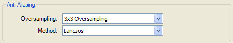
This improves the quality of the resulting image but dramatically increases the space required for sample data and the time required to compute it. Note that 3x3 Oversampling is over twice as costly as 2x2 Oversampling so plan accordingly.

Also, at this time you could try applying an Embossing or Sharpening filter to see how they look too. Both of these are found on the General properties page too.