
Fractal Programming Tutorial Overview
Fractal Programs are composed of a set of statements called Instructions. The Instructions are written in a language that is similar to the C programming language. The Programming Language supports a complete set of control structures including if statements, while loops, for loops, switch statements, inline functions/methods, arrays, and user defined objects. The complex data type is the fundamental variable type, and arithmetic operators and functions handle complex operands/arguments. A rich set of built-in functions/methods are included, and you can develop your own library of functions/methods for use throughout the application.
In addition to general programming support, the Fractal Science Kit supports a set of constructs used to define the properties pages associated with your programs. The user can interactively change the values of the properties on the properties pages to control program execution. Program Properties include enums, function proxies, option maps, options, option arrays, constants, and data tables.
In this tutorial we will examine 2 types of programs; Fractal Equations and Orbital Equations. These are the instructions that define the fractal iteration and are fundamental to understanding a fractal. Fractal Equations are the programs used to define Mandelbrot / Julia / Newton Fractals, and Orbital Equations are the programs used to define Orbital / IFS / Strange Attractor Fractals. Other Program Types supported by the Fractal Science Kit include Data Collection Programs, Color Controllers, and Complex Transformations.
You should work through the Fractal Equations section of this tutorial before you move on to the Orbital Equations section since these have been structured to build on one another.
This tutorial is a little different than the other Tutorials. While those concentrate on navigating the Properties Pages hierarchy, learning about key properties, and using the Built-in Programs to generate a variety of fractals, this tutorial introduces you to the key concepts involved in writing your own fractal programs. The descriptions given in this tutorial are not as detailed as those in the other Tutorials and I recommend that you work through those first so that you have a basic understanding of the application windows and the property page hierarchy. At a minimum, you should read the 1st page of the Tutorials which contains basic concepts required in the following sections.
Fractal Equations
Fractal Equations are the programs used to define Mandelbrot / Julia / Newton Fractals. In this section of the tutorial you will learn the basic structure of these programs and how to create/edit your own equations.
To begin, execute the Reset to Defaults command on the File menu of the Fractal Window.
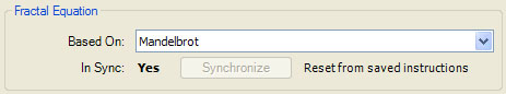
Open the Properties Window and select the Fractal Equation: Mandelbrot properties page:
General
Mandelbrot / Julia / Newton
Fractal Equation: Mandelbrot
This page is a Program Editor for the Fractal Equation. The Program Editor allows you to view/edit a program's Instructions, modify a program's properties, or to choose a different program altogether.
The program instructions are found in the editor pane at the bottom of the window. The editor pane is a simple text editor with support for standard commands like Undo, Redo, Cut, Copy, Paste, Delete, Select All, Clear All, and Find and Replace... along with a few additional commands useful for editing program instructions including Increase Indent, Decrease Indent, Comment Block, and Uncomment Block. See Editing Text for details.
Click the Toggle Code View button (2nd button from the left at the top of the page) on the Program Editor.
The Toggle Code View button hides the sections in the middle of the page containing the program's properties and expands the program's instructions to fill the space. This is called Code View. Clicking Toggle Code View again, restores the visibility of the sections in the middle of the page and shrinks the program's instructions to make room. Toggle Code View is useful when you are primarily concerned with viewing/editing the program's instructions. When Code View is active, the Toggle Code View toolbar button is depressed.
The editor pane contains the following program:
comment:
The classic Mandelbrot fractal discovered
in 1979 by Benoit B. Mandelbrot.
For details see the book:
"The Science of Fractal Images"
by M.F. Barnsley, R.L. Devaney, B.B. Mandelbrot,
H.-O. Peitgen, D. Saupe, R.F. Voss, with contributions
by Y. Fisher, M. McGuire.
Also see:
http://mathworld.wolfram.com/MandelbrotSet.html
http://en.wikipedia.org/wiki/Mandelbrot_set
http://classes.yale.edu/fractals/
iterate:
z = z^2 + c
These instructions are used to produce a classic Mandelbrot fractal or any of the related Julia fractals. The variables c and z are initialized by the Fractal Science Kit framework just before beginning each orbit, based on the type of fractal you are producing (Mandelbrot or Julia). For Julia fractals the framework assigns the Julia Constant to c and the pixel value to z. For Mandelbrot fractals the framework assigns the pixel value to c and the Initial Z value to z. See Mandelbrot / Julia / Newton Fractals for details.
A separate set of instructions is not required for Julia fractals. The choice of Mandelbrot or Julia is made simply by checking the Julia checkbox and setting the Julia Constant. The Fractal Science Kit will initialize z and c to the appropriate values based on these settings prior to invoking your instructions. Even checking the Julia checkbox and setting the Julia Constant is handled for you if you use the Preview Julia feature and simply click on an existing Mandelbrot display to select the Julia Constant.
Instructions are divided into sections. Each section begins with a section label which names the section. Each section performs a specific task related to the overall production of the fractal. The framework executes the code within a section at well-defined points within the fractal generation processing. This design is very powerful as it allows the framework to handle the common tasks necessary to generate a fractal while providing the developer a way to hook into the framework at critical points to perform tasks unique to the fractal at hand.
Section labels are placed alone on a line with no leading spaces and contain the section name followed by a colon (:). The instructions after a section label up until the next section label, define that section.
This program defines 2 sections; a comment section and an iterate section. Other sections that may be included in Fractal Equations include macros, global, initialize, and properties.
The comment section is a place to provide usage instructions, hints, notes, documentation of the code, etc. The compiler ignores the comment section altogether.
The initialize section is executed just prior to beginning each orbit. Instructions that need to execute at the beginning of each orbit should be placed there. This program does not require an initialize section.
The iterate section is executed during the fractal iteration to generate the orbit points. The variable z holds the orbit point. The job of the iterate section is to set z to the value of the next orbit point.
In this example, the iterate section is a single assignment.
iterate:
z = z^2 + c
This statement takes 2 complex values found in the variables z and c, and combines them based on the expression to the right of the equal sign; in this case, by squaring z and adding c to the result. The resulting complex value is assigned to the variable z, replacing the previous value of z.
The macros section, global section, and properties section are discussed later.
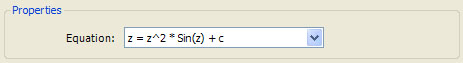
Change the assignment in the iterate section to:
z = z^2 * Sin(z) + c
Execute the Display Fractal command on the Tools menu of the Fractal Window to generate the fractal image based on the new equation.
Here are some other equations you can try:
- z = z^2 * Sin(z) + c
- z = z^2 * Cos(z) + c
- z = z^2 * Tan(z) + c
- z = z^2 * Sin(z)^2 + c
- z = z^2 * Cos(z)^2 + c
- z = z^2 * Tan(z)^2 + c
Of course, not all equations produce nice images but it is easy try out any equation you can imagine. Changes to some of the other properties on this page (Initial Z, Max Power, Power Factor) are required for some equations to get the best results. See Fractal Equations for details.
Now let's see how we can set up a single program to handle all of the above equations.
First, clear the existing program text. To do this, right-click on the editor pane and click the Clear All command.
Next, copy the following program into the editor pane:
iterate:
switch (Equation) {
case EquationTypes.Eq1: z = z^2 * Sin(z) + c
case EquationTypes.Eq2: z = z^2 * Cos(z) + c
case EquationTypes.Eq3: z = z^2 * Tan(z) + c
case EquationTypes.Eq4: z = z^2 * Sin(z)^2 + c
case EquationTypes.Eq5: z = z^2 * Cos(z)^2 + c
case EquationTypes.Eq6: z = z^2 * Tan(z)^2 + c
}
properties:
enum EquationTypes {
Eq1, "z = z^2 * Sin(z) + c"
Eq2, "z = z^2 * Cos(z) + c"
Eq3, "z = z^2 * Tan(z) + c"
Eq4, "z = z^2 * Sin(z)^2 + c"
Eq5, "z = z^2 * Cos(z)^2 + c"
Eq6, "z = z^2 * Tan(z)^2 + c"
}
option Equation {
type = EquationTypes
caption = "Equation"
default = EquationTypes.Eq1
}
This program includes an iterate section and a properties section. Let's discuss the properties section first.
The properties section is used to define the properties pages associated with the program. Most of the statements in this section result in one or more constants that you will use in the other sections of your program to control program flow. The user interacts with the properties on the properties pages which sets the values of the constants used by the other sections of your program. Expressions using these constants are highly optimized resulting in much faster execution times.
This program defines a single properties page with a single property called Equation as an enum option.
An enum option is used when the data represents a single value from a set of choices. You need to define an enum using an Enum Statement before you define an enum option. The enum statement defines a set of enum items. Each item defines an identifier and a string that represents the item to the user on the properties page.
Next, you define an enum option and set the option's type field to the enum name, EquationTypes in our example. The option's default field should be set to one of the values associated with the named enum. The default is given as the enum name followed by a period (.) and the enum item name. This is also how the enum item is referenced in your program. The enum option is typically used with a switch statement in the program instructions. A combobox is provided for user input. See Enum Statement for details.
Click the Refresh Properties Pages button (the 3rd button from the left at the top of the page) on the Program Editor to view the Properties item in the page hierarchy to the left and then select the Properties item to view the properties page:
The user can select one of the equation types using the combobox and the program instructions use this information to control the program processing as shown in the iterate section below:
iterate:
switch (Equation) {
case EquationTypes.Eq1: z = z^2 * Sin(z) + c
case EquationTypes.Eq2: z = z^2 * Cos(z) + c
case EquationTypes.Eq3: z = z^2 * Tan(z) + c
case EquationTypes.Eq4: z = z^2 * Sin(z)^2 + c
case EquationTypes.Eq5: z = z^2 * Cos(z)^2 + c
case EquationTypes.Eq6: z = z^2 * Tan(z)^2 + c
}
Here a switch statement based on the Equation property controls which equation to execute during the fractal iteration. In fact, since Equation is a constant, the compiler will evaluate the switch statement during Program Optimization and the switch statement processing is entirely eliminated in the optimized code.
Experiment with the program by changing the program properties and executing the Display Fractal command on the Tools menu of the Fractal Window to generate the fractal image.
Now let's try an alternate approach to the same problem.
Clear the existing program text and copy the following program into the editor pane:
iterate:
z = z^2 * F(z)^P + c
properties:
divider {
caption = "z = z^2 * F(z)^P + c"
}
functionSet Functions {
Sin Cos Tan
}
option F {
type = Functions
caption = "F"
default = Sin
}
option P {
type = IntegerEnum(1, 6)
caption = "P"
default = 1
}
This program provides essentially the same functionality as the previous program but using a different set of properties.
Here we define 2 options; a function proxy (F) and an integer enum (P):
A function proxy is an option that represents a function. In your code, you invoke a function proxy just like you invoke a function except that the name of the function is the proxy name. The compiler replaces the function proxy with the actual function at compile time. A functionSet statement is used to create a list of functions that can be associated with a function proxy.
We define a function proxy F that can be set to one of the functions: Sin, Cos, or Tan.
An integer enum option is used for integral data. It creates a small combobox with a list of integers from which to choose and can be used when the range of integers associated with an option is small.
We define an integer enum P that holds an integer between 1 and 6 inclusive.
Select the Properties item to view the properties page:
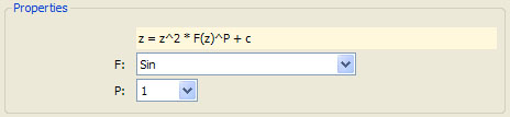
The user can change the equation by selecting different values for F and/or P and the program instructions use this information to control the program processing as shown in the iterate section below:
iterate:
z = z^2 * F(z)^P + c
The compiler will replace F with the selected function, and P with the selected integer before executing the program.
Experiment with the program by changing the program properties and executing the Display Fractal command on the Tools menu of the Fractal Window to generate the fractal image.
For more information relating to the programs that define Mandelbrot / Julia / Newton Fractals, see Fractal Equations.
Orbital Equations
Orbital Equations are the programs used to define Orbital / IFS / Strange Attractor Fractals. In this section of the tutorial you will learn the basic structure of these programs and how to create/edit your own equations.
To begin, execute the Reset to Defaults command on the File menu of the Fractal Window.
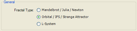
Open the Properties Window and select the General properties page:
Select Orbital / IFS / Strange Attractor for the Fractal Type in the General section of the page.
Next, turn on Anti-Aliasing by setting Oversampling to 2x2 Oversampling in the Anti-Aliasing section.
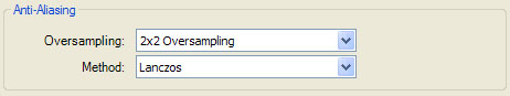
This dramatically increases the space required for sample data and the time required to compute it, and should be used with care. However, since Orbital fractals do not generate an orbit per sample as do Mandelbrot fractals, anti-aliasing does not result in as severe a time penalty as with Mandelbrot fractals, and it is recommended that you set Oversampling to one of the higher settings when exploring Orbital fractals since the increased quality outweighs the cost.
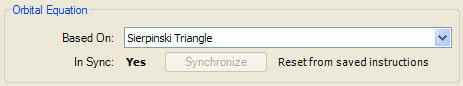
Next, select the Orbital Equation: Sierpinski properties page:
General
Orbital / IFS / Strange
Attractor
Orbital Equation: Sierpinski
This page is a Program Editor for the Orbital Equation. The Program Editor allows you to view/edit a program's Instructions, modify a program's properties, or to choose a different program altogether.
The program instructions are found in the editor pane at the bottom of the window.
The editor pane contains the following program:
comment:
This program generates a Sierpinski Triangle.
This fractal was described by Waclaw Sierpinski
in 1915!
The fractal exterior is an equilateral triangle.
The options Center and Radius control the size
and position of the triangle's circumcircle.
The Angle option is used to rotate the triangle
counterclockwise.
On each iteration, we select a vertex of the
equilateral triangle at random and move the
orbit point to the midpoint of the segment that
connects the current point to the selected vertex.
For details see:
http://mathworld.wolfram.com/SierpinskiSieve.html
http://en.wikipedia.org/wiki/Sierpinski_triangle
global:
const Complex point[3]
Geometry.GeneratePointsOnCircle( \
point[], 3, Center, Radius, DegreeToRadian(Angle) \
)
iterate:
attractorIndex = Random.Integer(3)
z = Geometry.MidPoint(z, point[attractorIndex])
properties:
option Center {
type = Complex
caption = "Center"
details = "Center of equilateral triangle"
default = 0
}
option Radius {
type = Float
caption = "Radius"
details = "Radius of triangle circumcircle"
default = 1
range = (0,)
}
option Angle {
type = Float
caption = "Angle"
details = "Angle of rotation"
default = 0
range = [-360,360]
}
These instructions are used to produce a Sierpinski Triangle.
This program defines 4 sections; a comment section, a global section, an iterate section, and a properties section. We have seen the comment, iterate, and properties sections in previous examples.
The global section is where you place program initialization statements. This section is executed exactly once, each time the program runs. This is where you should initialize data structures, declare arrays, perform one time calculations, etc. Since this section is executed only once, compared to other sections that are executed many times during the program's execution, you should try to move as much processing into the global section as possible.
- The global section is also where all constants (i.e., variables declared const) must be declared and initialized. You can assign a value to a variable declared const anywhere inside the global section, just like any other variable. However, in the program's other sections, constants cannot be changed, and expressions using constants are highly optimized resulting in much faster execution times. Clearly, any variable that is initialized in the global section, and used, but not changed, in other sections, should be declared as const.
Here, we create/initialize an array called point[] that holds the coordinates of the vertices of an equilateral triangle with the Center, Radius, and Angle of rotation taken from the defined properties. This is achieved by calling the inline function Geometry.GeneratePointsOnCircle defined in the Built-in Macros. The built-in macros provide access to large set of useful Inline Functions and Inline Methods, and you can develop your own library of functions/methods for use throughout the application as well.
For reference, here is the source for the Geometry.GeneratePointsOnCircle method:
'
' This method fills points[] with count points equally spaced
' around a circle with the given center and radius, and starting
' with a point at angle angle0 radians around the circle. The array
' points[] is assumed to be large enough to hold count values.
'
void Geometry.GeneratePointsOnCircle( \
points[], count, center, radius, angle0 \
) {
if (count > 0) {
inc = 2*Math.PI/count
ang = angle0
for (i = 0, i < count, i += 1) {
points[i] = center + radius*Cis(ang)
ang += inc
}
}
}
The arguments to this method include the array used to return the points on the circle (points[]), the number of points to generate (count), and the center, radius, and starting angle of the 1st point (angle0). The comments above the function definition describe its operation.
In the global section of our program, we dimension an array to hold the 3 vertices of the triangle and call the Geometry.GeneratePointsOnCircle method using the properties defined in the properties section: Center, Radius, and Angle. Center is a complex number and Radius and Angle are floats, each with a restricted range given by the associated range parameter assignments. Radius is required to be greater than 0 and Angle must be between -360 and 360 inclusive.
The iterate section is executed during the fractal iteration to generate the orbit of the Orbital equation.
The iterate section of our program is defined as:
iterate:
attractorIndex = Random.Integer(3)
z = Geometry.MidPoint(z, point[attractorIndex])
On each iteration, one of the triangle's vertices is selected at random, and the point z is shifted to the midpoint of the segment connecting the previous value of z and the selected vertex.
The variables z and attractorIndex are used to return the results computed by the Orbital Equation. z is the value computed for the next orbit point. attractorIndex is an index between 0 and 255 that is mapped to the sample point's AttractorIndex field which can be used by the color controller (the program that maps the fractal's data to colors) to assign a color to the sample. Typically, as in this example, attractorIndex is an index identifying which attractor influenced z on this iteration. z is responsible for the shape of the fractal and attractorIndex is responsible for the color.
Select the Properties item to view the properties page:
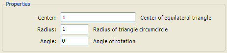
The user can control the equation by selecting different values for Center, Radius, and Angle.
Experiment with the program by changing the program properties and executing the Display Fractal command on the Tools menu of the Fractal Window to generate the fractal image.
Now let's change the program to allow the user to specify the number of vertices in the generating polygon.
Change the properties section as shown below:
properties:
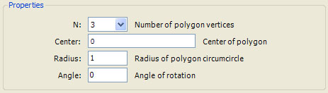
option N {
type = IntegerEnum(3, 6)
caption = "N"
details = "Number of polygon vertices"
default = 3
}
option Center {
type = Complex
caption = "Center"
details = "Center of polygon"
default = 0
}
option Radius {
type = Float
caption = "Radius"
details = "Radius of polygon circumcircle"
default = 1
range = (0,)
}
option Angle {
type = Float
caption = "Angle"
details = "Angle of rotation"
default = 0
range = [-360,360]
}
Here we have added the integer enum N and changed the details field for Center and Radius.
Change the global section as shown below:
global:
const Complex point[N]
Geometry.GeneratePointsOnCircle( \
point[], N, Center, Radius, DegreeToRadian(Angle) \
)
This is identical to the previous example except that we have changed the 3 to N in the array declaration and the 2nd argument to Geometry.GeneratePointsOnCircle.
Change the iterate section as shown below:
iterate:
attractorIndex = Random.Integer(N)
z = Geometry.MidPoint(z, point[attractorIndex])
Here too, we have changed the 3 to N in the argument to Random.Integer.
Here is the entire program for reference:
global:
const Complex point[N]
Geometry.GeneratePointsOnCircle( \
point[], N, Center, Radius, DegreeToRadian(Angle) \
)
iterate:
attractorIndex = Random.Integer(N)
z = Geometry.MidPoint(z, point[attractorIndex])
properties:
option N {
type = IntegerEnum(3, 6)
caption = "N"
details = "Number of polygon vertices"
default = 3
}
option Center {
type = Complex
caption = "Center"
details = "Center of polygon"
default = 0
}
option Radius {
type = Float
caption = "Radius"
details = "Radius of polygon circumcircle"
default = 1
range = (0,)
}
option Angle {
type = Float
caption = "Angle"
details = "Angle of rotation"
default = 0
range = [-360,360]
}
Select the Properties item to view the properties page:
Experiment with the program by changing the program properties and executing the Display Fractal command on the Tools menu of the Fractal Window to generate the fractal image.
Now let's define a fractal based on 2 affine transformations.
Clear the existing equation and copy/paste the following text into the editor pane:
global:
factor = Sqrt(2)/2
ang1 = DegreeToRadian(A1)
ang2 = DegreeToRadian(A2)
Affine T1 = Affine.Identity()
Affine.Scale(T1, factor)
if (R1) {
Affine.ReflectAboutXAxis(T1)
}
Affine.Rotate(T1, ang1)
Affine.Translate(T1, Complex(1, 0))
Affine T2 = Affine.Identity()
Affine.Scale(T2, factor)
if (R2) {
Affine.ReflectAboutXAxis(T2)
}
Affine.Rotate(T2, ang2)
Affine.Translate(T2, Complex(-1, 0))
const Affine s[] = T1, T2
iterate:
attractorIndex = IIf(Random.Number() < Weight, 0, 1)
z = Affine.TransformPoint(s[attractorIndex], z)
properties:
optionMap Dimers(A1, R1, A2, R2) {
Custom,
"<Custom>",
0, False, 0, False
Rectangle,
"Rectangle",
90, False, 90, False
Twindragon,
"Twindragon",
45, False, 45, False
Parallelogram,
"Parallelogram", 60,
True, 60, True
HarterHeighwayDragon, "Harter-Heighway Dragon", 45,
False, 135, False
CesaroTriangle, "Cesaro
Triangle", 135, False, 225, False
Scorpion,
"Scorpion",
45, True, 315, False
Arachnodragon, "Arachnodragon",
135, True, 225, False
LevyDragon,
"Levy Dragon",
315, False, 45, False
Dibolt,
"Dibolt",
45, True, 135, True
}
option Dimer {
type = Dimers
caption = "Dimer"
default = Dimers.HarterHeighwayDragon
}
divider {
caption = "Transformation 1"
}
option A1 {
type = Float
caption = "Rotation"
details = "Angle of rotation"
default = 0
range = [-360,360]
}
option R1 {
type = Boolean
caption = "Reflection"
details = "Include reflection about X axis"
default = False
}
divider {
caption = "Transformation 2"
}
option A2 {
type = Float
caption = "Rotation"
details = "Angle of rotation"
default = 0
range = [-360,360]
}
option R2 {
type = Boolean
caption = "Reflection"
details = "Include reflection about X axis"
default = False
}
divider {
caption = "General"
}
option Weight {
type = Float
caption = "Weight"
details = "Weight assigned to 1st transformation (0-1)"
default = 0.4
range = [0,1]
}
This program defines 2 affine transformations. Each transformation is defined by a fixed contractive scaling, a rotation, an optional reflection about the X axis, and a translation. On each iteration, one of the transformations is selected at random based on a user specified weight, and the selected transformation is used to transform the orbit point.
The properties section defines the program's parameters.
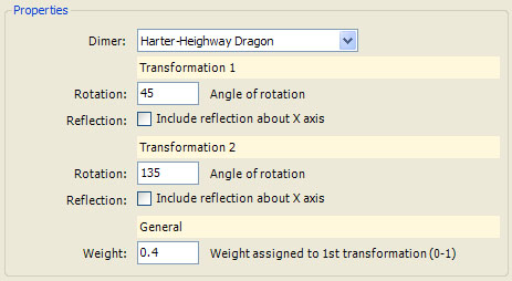
The options A1 and A2 control the angle of rotation for the 2 transformations, respectively. The options R1 and R2 are Boolean Options that control an optional reflection about the X axis applied to each transformation. The Weight option allows the user to control the probability of selecting the 1st transformation when a random transformation is selected within the fractal iteration. Also, note the use of the Divider Statement to separate the options into groups.
Finally, note the use of the OptionMap Statement to predefine a set of examples:
optionMap Dimers(A1, R1, A2, R2) {
Custom,
"<Custom>",
0, False, 0, False
Rectangle,
"Rectangle",
90, False, 90, False
Twindragon,
"Twindragon",
45, False, 45, False
Parallelogram,
"Parallelogram", 60,
True, 60, True
HarterHeighwayDragon, "Harter-Heighway Dragon", 45,
False, 135, False
CesaroTriangle, "Cesaro
Triangle", 135, False, 225, False
Scorpion,
"Scorpion",
45, True, 315, False
Arachnodragon, "Arachnodragon",
135, True, 225, False
LevyDragon,
"Levy Dragon",
315, False, 45, False
Dibolt,
"Dibolt",
45, True, 135, True
}
option Dimer {
type = Dimers
caption = "Dimer"
default = Dimers.HarterHeighwayDragon
}
An option map option is used to create named sets of related options that can be set by selecting the name from a combobox. When an item is selected, all the component options are updated with the values specified in the associated OptionMap Statement. The user can accept the set of values as is, or change one or more of the component values. This provides the user with a set of example parameter sets while still allowing the user to try new parameter sets not specified in the OptionMap Statement. You need to define an optionMap (using an OptionMap Statement) before you define the option map option. Then you set the option's type field to the optionMap name. The option's default field should be set to one of the values associated with the named optionMap. The default is given as the optionMap name followed by a period (.) and the optionMap item name. All of the values associated with the the option map option's default override the default values for the associated options. See OptionMap Statement for details.
Here we define a collection of dimers from Stewart R. Hinsley's Dimers(2D) site.
The global section is where we define the 2 affine transformations based on the property settings:
global:
factor = Sqrt(2)/2
ang1 = DegreeToRadian(A1)
ang2 = DegreeToRadian(A2)
Affine T1 = Affine.Identity()
Affine.Scale(T1, factor)
if (R1) {
Affine.ReflectAboutXAxis(T1)
}
Affine.Rotate(T1, ang1)
Affine.Translate(T1, Complex(1, 0))
Affine T2 = Affine.Identity()
Affine.Scale(T2, factor)
if (R2) {
Affine.ReflectAboutXAxis(T2)
}
Affine.Rotate(T2, ang2)
Affine.Translate(T2, Complex(-1, 0))
const Affine s[] = T1, T2
Based on the options A1, A2, R1, and R2, we create the 2 affine transformations T1 and T2 and assign them to an array of affine transformations called s[].
An affine transformation Object is defined in the Built-in Macros as:
Object Affine {
A
B
C
D
E
F
}
This defines an Affine object with 6 members: A, B, C, D, E, and F. These members can be accessed by giving the variable name followed by a period (.) and the object member name.
Example:
z = Complex( \
t.A*z.x + t.B*z.y + t.E, \
t.C*z.x + t.D*z.y + t.F \
)
This example transforms a point z based on an Affine transformation object named t.
This is equivalent to the following:
z = Affine.TransformPoint(t, z)
This example uses one of the Affine Functions defined in the Built-in Macros to transform the point.
A few of the Affine Functions used by our program are included below for reference:
'
' Return the identity transformation.
'
Affine Affine.Identity() = Affine(1, 0, 0, 1, 0, 0)
'
' Affine.TransformPoint applies an affine transformation
' matrix to a point z and returns the resulting point.
'
' A B E z.X A*z.X + B*z.Y + E
' C D F * z.Y = C*z.X + D*z.Y + F
' 0 0 1 1 1
'
Complex Affine.TransformPoint(Affine a, z) {
return Complex( \
a.A*z.x + a.B*z.y + a.E, \
a.C*z.x + a.D*z.y + a.F \
)
}
'
' Inject a translation by shift into the given
' affine transformation.
'
' 1 0 shift.X A B E A B
E+shift.X
' 0 1 shift.Y * C D F = C D F+shift.Y
' 0 0 1 0 0 1
0 0 1
'
void Affine.Translate(byref Affine a, shift) {
a.E = a.E + shift.x
a.F = a.F + shift.y
}
'
' Inject a rotation by angle radians ccw into the given
' affine transformation.
'
' Ca -Sa 0 A B E Ca*A-Sa*C
Ca*B-Sa*D Ca*E-Sa*F
' Sa Ca 0 * C D F = Sa*A+Ca*C Sa*B+Ca*D Sa*E+Ca*F
' 0 0 1 0 0 1
0 0
1
'
' where Ca = Cos(angle) and Sa = Sin(angle)
'
void Affine.Rotate(byref Affine a, angle) {
Ca = Cos(angle)
Sa = Sin(angle)
tmp = Ca*a.A - Sa*a.C
a.C = Sa*a.A + Ca*a.C
a.A = tmp
tmp = Ca*a.B - Sa*a.D
a.D = Sa*a.B + Ca*a.D
a.B = tmp
tmp = Ca*a.E - Sa*a.F
a.F = Sa*a.E + Ca*a.F
a.E = tmp
}
'
' Inject a scaling by S into the given
' affine transformation.
'
' S.y = 0:
'
' S 0 0 A B E S*A S*B S*E
' 0 S 0 * C D F = S*C S*D S*F
' 0 0 1 0 0 1 0 0
1
'
' S.y <> 0:
'
' S.x 0 0 A B E S.x*A S.x*B
S.x*E
' 0 S.y 0 * C D F = S.y*C S.y*D S.y*F
' 0 0 1 0 0 1 0
0 1
'
void Affine.Scale(byref Affine a, S) {
if (S.y = 0) {
a.A = S*a.A
a.C = S*a.C
a.B = S*a.B
a.D = S*a.D
a.E = S*a.E
a.F = S*a.F
} else {
a.A = S.x*a.A
a.C = S.y*a.C
a.B = S.x*a.B
a.D = S.y*a.D
a.E = S.x*a.E
a.F = S.y*a.F
}
}
'
' Inject a reflection about the X axis into
' the given affine transformation.
'
' 1 0 0 A B E
A B E
' 0 -1 0 * C D F = -C -D -F
' 0 0 1 0 0 1
0 0 1
'
void Affine.ReflectAboutXAxis(byref Affine a) {
a.C = -a.C
a.D = -a.D
a.F = -a.F
}
See the discussion of Inline Functions and Inline Methods for general information about writing inline functions/methods.
Now we come at last to the fractal iteration code:
iterate:
attractorIndex = IIf(Random.Number() < Weight, 0, 1)
z = Affine.TransformPoint(s[attractorIndex], z)
Here we generate a random number between 0 and 1, and compare it to the Weight option specified by the user. If the number is less than Weight we set attractorIndex to 0. Otherwise, we set attractorIndex to 1. To code this, we use the IIf statement:
IIf(<Condition>, <Value-If-True>, <Value-If-False>)
The IIf function evaluates the conditional expression and evaluates/returns 1 of the 2 expressions based on the result. IIf is handled differently than other functions in that only 1 of the expressions <Value-If-True> or <Value-If-False> is evaluated, depending on the conditional expression. Contrast this with the way all other functions are invoked where we evaluate all the function's arguments before calling the function. IIf can return an object or a complex number but <Value-If-True>, <Value-If-False>, and the variable to which the function result is assigned, must all be the same type.
Finally, we use attractorIndex as an index into the array s[] and use the resulting affine transformation to transform z.
Experiment with the program by changing the program properties and executing the Display Fractal command on the Tools menu of the Fractal Window to generate the fractal image.
For more information relating to the programs that define Orbital / IFS / Strange Attractor Fractals see Orbital Equations.
This concludes the fractal programming tutorial. For additional details see the Programming Language section of the documentation.