
<Back> 1 2 3 4 5 6 7 8 9 <Next>
In Part 9 of the tutorial, we will learn how to use the Complex Grid orbit trap as a visualization aid for Complex Analysis, the branch of mathematics studying functions of a complex variable. We will use the Composite Function transformation to apply a composite function to each point on the complex plane and color the image based on the transformed point's angle or magnitude. On top of this base image we will display the Complex Grid trap.
The Complex Grid trap displays a grid made up of horizontal and vertical lines equally spaced across the complex plane. We color each point on the grid based on the point's angle relative to the grid origin. The Complex Grid trap gives additional cues as to how the transformation warps the complex plane.
Execute the Reset to Defaults command on the File menu of the Fractal Window.
Select the General properties page:
Turn on Anti-Aliasing by setting Oversampling to 2x2 Oversampling in the Anti-Aliasing section.
![]()
This increases the space required for sample data and the time required to compute it, but in this case, it is required since the grid lines can become very thin based on the transformation in effect. Since we do not need to run the fractal iteration for this example, the processing time is not too bad.
Next, select the Mandelbrot / Julia / Newton properties page:
General
Mandelbrot / Julia / Newton
Set Type to Both in the Mandelbrot / Julia/ Newton section of the page.

This allows us to overlay the orbit trap on top of the base image generated by the classic subsystem.
Set Bailout to 1e16 in the Orbit Generation section of the page:
![]()
The reason we do this is to ensure points with large magnitudes are processed. Some of the transformations map 1 or more points on the complex plane to infinity. A point z such that f(z) maps to infinity is called a pole with respect to the function f. The value of f(z) for points on the complex plane near these poles have very large magnitudes. The image generation subsystem terminates processing if the orbit point is greater than Bailout so to ensure we process points near the poles we need to set Bailout to a large number.
Select the Fractal Equation: Mandelbrot properties page:
General
Mandelbrot / Julia / Newton
Fractal Equation: Mandelbrot
This page is a Program Editor for the Fractal Equation.
Change the Based On property to Pixel. Pixel is at the end of the list of built-in equations.
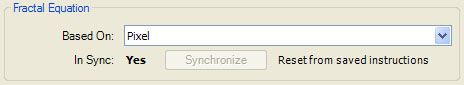
This Fractal Equation eliminates the fractal iteration altogether and simply returns the pixel value for the point.
Now we need to define an Alternate Mapping to hold each point's angle/magnitude.
Select the Alternate Mapping 1: <None> properties page:
General
Mandelbrot / Julia / Newton
Alternate Mapping 1: <None>
Set the Type to Instructions.

When you set the mapping to Instructions, a Program Editor for an Alternate Value is displayed in the page hierarchy under the Alternate Mapping page. This setting is the most flexible since it provides you with full control over the data collection processing.
The default Alternate Value is Orbit Point which saves the polar coordinates of the last orbit point in the sample's fields Alternate 1 Value and Alternate 1 Angle. Alternate 1 Value is the point's magnitude (i.e., the distance from the origin) and Alternate 1 Angle is the point's argument (i.e., the angle relative to the X axis). Since we are using the Fractal Equation Pixel, the point is the transformed pixel value. This is exactly what we need.
Set the Method property to Inside/Outside Together.
![]()
Mandelbrot samples can be categorized by whether or not the associated orbit diverged (or converged if the fractal type is Convergent). If the orbit diverged (or converged), the sample is said to be outside the Mandelbrot set. Otherwise, it is said to be inside the set. Normalization can be applied to the sample data using 2 different methods: Inside/Outside Together or Inside/Outside Separately. The 1st method normalizes all the sample values in a single group. The 2nd method normalizes the inside samples separately from the outside samples. In this case, each of the 2 sets has a different set of normalization control parameters.
Since we are not performing the fractal iteration, the concept of inside/outside points is meaningless, and we need to set the Method property to Inside/Outside Together so that normalization processes all the sample values in a single group.
Check both Max Cutoff Value and the Use percentile (0 - 100) checkbox to its right, and enter 99 in the Max Cutoff Value textbox.
![]()
This is done to eliminate outlier data values from consideration while normalizing the data. This is required since some of the transformations map 1 or more points on the complex plane to infinity and the magnitude of (transformed) points near these poles would thwart normalization efforts. These settings ignore the top 1% of the values when normalizing the data.
Next, select the (Classic) Gradient Map - Value properties page:
General
Mandelbrot / Julia / Newton
Classic
Controllers
Gradient Map - Value
This page is a Program Editor for the Classic Controller.
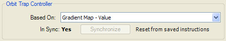
Change the Based On property to Gradient Map - Complex Analysis.

Select the program's Properties page (found below the controller in the hierarchy) and change Color Scheme to 4 Bars - Purple, Silver, Red, Gold.

The Color Scheme setting allows you to choose 1 of the gradients included in the controller's gradient list.
The Color Map property controls the data used to index into the gradient and can be either Angle or Magnitude.
![]()
The Angle setting maps the transformed point's angle to the gradient index. The Magnitude setting maps the transformed point's magnitude to the gradient index. Each of these provide helpful cues when visualizing the effects of the transformation on the points on the complex plane.
Due to the nature of the gradient we assigned to Color Scheme, the Angle setting will color each of the 4 quadrants with a different color. This allows you to determine how the transformation affects points in each of the 4 quadrants.
Leave the Color Map set to Angle (the default). Later you can return to this page and try the Magnitude setting.
Next, select the Instructions: Circle properties page:
General
Mandelbrot / Julia / Newton
Orbit Trap
Orbit Trap Map
Instructions: Circle
This page is a Program Editor for the Orbit Trap.
Change the Based On property to Complex Grid.
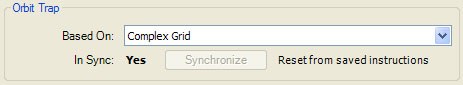
Select the program's Properties page.
Note the Type property is Square by default, but can be set to any of the following:
- Square
- Square (Open Center)
- Square (Brick)
- Weave
- Polar
- Polar (Open Center)
- Polar (Brick)
![]()
We will use the default type (Square). Later, you can return to this page and experiment with the other grid types.
Next, select the (Orbit Trap) Gradient Map - Value properties page:
General
Mandelbrot / Julia / Newton
Orbit Trap
Controllers
Gradient Map - Value
This page is a Program Editor for the Orbit Trap Controller.
In the 3D Mapping section, check Apply Depth.
![]()
This adds a metallic quality to the resulting colors.
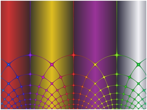
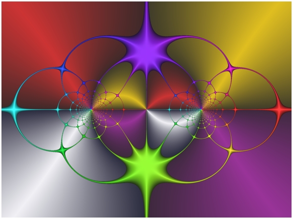
Execute the Display Fractal command on the Tools menu of the Fractal Window to generate the fractal image.
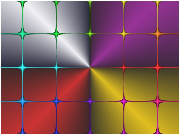
This is the base image without any transformations applied. Note how the 4 quadrants of the base image are colored purple, silver, red, and gold, respectively, and the Complex Grid is colored based on the angle of the point relative to the origin.
Now, let's set up a transformation.
Select the Transformation properties page:
General
Mandelbrot / Julia / Newton
Transformation
This page allows you to maintain a list of Transformations used to transform the pixel prior to starting each orbit. The transformations are applied in series to the pixel value; i.e., the point resulting from each transformation is passed to the next transformation in the list. As you will see, this can have a dramatic effect on the resulting image. By default, there is a single transformation, Identity, and the Identity transformation does not alter the input point.
Select the Identity properties page:
General
Mandelbrot / Julia / Newton
Transformation
Identity
This page is a Program Editor for a Transformation.
We want to use the Composite Function transformation so we set the Based On property to that.
![]()
Select the program's Properties page just below the transformation in the hierarchy:
General
Mandelbrot / Julia / Newton
Transformation
Composite Function
Properties
This displays the default properties for the Composite Function transformation. The Composite Function transformation is defined by a composite function composed of 2 functions. Each function is defined via a base function and a conjugating map. For now, we will only set the F(z) and/or G(z) properties and leave the remaining properties set to their default value.
Try setting F(z) and/or G(z) to different functions and then execute the Display Fractal command on the Tools menu of the Fractal Window.
A few examples are shown below:
|
|
|
|
|
|
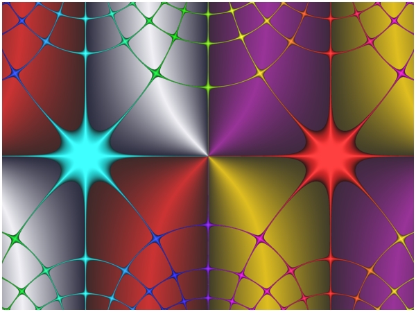
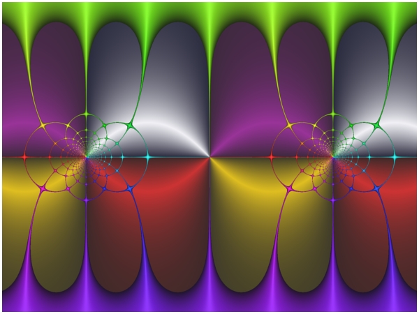
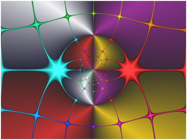

G(z) is set to Ident in the above examples.
This concludes the Orbit Trap tutorial. Click <Next> to continue with the Orbital Fractals Tutorial.