
Fractal Equations Overview
Fractal Equations are the programs used to define Mandelbrot Fractals in the Fractal Science Kit fractal generator. Before you begin, please read the Mandelbrot Fractal Overview.
See also:
- Mandelbrot Fractal Overview
- Base Equations
- Properties Window
- Program Editors
- Fractal Programs
- Program Instructions
- Programming Language
Each program is composed of a set of properties and instructions.
Comments
Always remember to click the Toggle Code View toolbar button at the top of the Program Editor and read the comments given in the comment section of the program's instructions. The comment section contains usage instructions, hints, notes, documentation, and other important information that will help you understand how best to use the program. Once you are done reading the comments, click the Toggle Code View toolbar button again to view the program's properties.
Properties
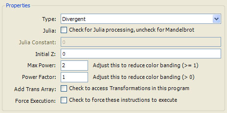
The following properties are supported:
-
Type can be set to Divergent, Convergent, or Convergent or Divergent and determines the method used to terminate the orbit iteration. Divergent fractals terminate the iteration when the magnitude exceeds the Bailout value in the Orbit Generation section of the Mandelbrot / Julia / Newton page. Convergent fractals terminate the iteration when the magnitude is less than the value Epsilon, also defined in the Orbit Generation section of the Mandelbrot / Julia / Newton page. Convergent or Divergent fractals terminate the iteration when either condition occurs. Type is closely related to the formula given in the instructions and a given formula will usually dictate which setting is required.
-
Julia is a checkbox that determines how the variables z and c are initialized at the beginning of each orbit. If Julia is checked, z is set to the pixel value associated with the orbit and c is set to the Julia Constant. If Julia is not checked, z is set to the Initial Z and c is set to the pixel value associated with the orbit. These differences characterize the fractal as a Julia fractal (if Julia is checked) or a Mandelbrot fractal (if Julia is not checked), respectively. You can use this checkbox to change a Mandelbrot fractal to a Julia fractal or vice versa but you will need to specify the Initial Z value for Mandelbrot fractals or the Julia Constant for Julia fractals, as well. It is usually easier to use the Preview Julia command on the Fractal Window to explore the different Julia fractals for a given Mandelbrot fractal.
-
Initial Z is a numeric textbox used to enter a complex value for the Initial Z required for Mandelbrot fractals. This property is disabled if the Julia checkbox is checked since Julia fractals do not require this value. If the initial z value is dependent on selected properties set by the user, you will need to initialize z in the initialize section of the program instructions and the Initial Z property can be ignored. See below for details.
-
Julia Constant is a numeric textbox used to enter a complex value for the Julia Constant required for Julia fractals. This property is disabled if the Julia checkbox is not checked since Mandelbrot fractals do not require this value. If you use the Preview Julia command on the Fractal Window to explore the different Julia fractals for a given Mandelbrot fractal, this property is set for you based on where you click on the associated Mandelbrot fractal.
-
Max Power and Power Factor are numeric textboxes used to enter values that can reduce color banding in some situations. For Mandelbrot Power equations of the form z=z^K+c, Max Power should be set to K. The rule of thumb is to set Max Power to the highest power of z used in the equation but this does not always work and you may need to fiddle with Max Power and/or Power Factor to reduce dwell based artifacts in the image.
-
Add Trans Array is a checkbox that can be checked to add a Transformation Array editor as one of the program's properties pages. Users can add 1 or more transformations to the editor and your program can access the transformations using the Transformation Functions.
-
Force Execution is a checkbox that can be checked to force execution of the instructions. If Force Execution is unchecked, the instructions will execute only if required based on what changes were made to the fractal's properties since the last time the instructions ran. This is rarely checked.
Instructions
The remainder of this page can be ignored if you are not a programmer.
At the bottom of the window is an editor pane named Instructions. The editor pane is a simple text editor to view/edit your Program Instructions. See Editing Text for details.
The instructions are divided into sections. Within each section are statements that conform to the Programming Language syntax.
In addition to the Standard Sections, Fractal Equations support 2 other sections:
initialize:
iterate:
The initialize section is executed once per pixel, just prior to beginning the orbit. Instructions that need to execute at the beginning of each orbit should be placed here. The iterate section is executed once per iteration and is the primary section of the fractal equation.
Example:
comment:
The classic Mandelbrot fractal discovered
in 1979 by Benoit B. Mandelbrot.
For details see the book:
"The Science of Fractal Images"
by M.F. Barnsley, R.L. Devaney, B.B. Mandelbrot,
H.-O. Peitgen, D. Saupe, R.F. Voss, with contributions
by Y. Fisher, M. McGuire.
Also see:
http://mathworld.wolfram.com/MandelbrotSet.html
http://en.wikipedia.org/wiki/Mandelbrot_set
http://classes.yale.edu/fractals/
iterate:
z = z^2 + c
These instructions can be used to produce a Mandelbrot fractal or any of the related Julia fractals. A separate set of instructions is not required for Julia fractals. The choice of Mandelbrot or Julia is made simply by checking the Julia checkbox and setting the Julia Constant. The Fractal Science Kit will initialize z and c to the appropriate values based on these settings prior to invoking your instructions. Even checking the Julia checkbox and setting the Julia Constant is handled for you if you use the Preview Julia feature and simply click on an existing Mandelbrot display to select the Julia Constant.
There is one situation where your code needs to be aware of which type (Mandelbrot or Julia) of fractal it is producing. If the instructions set the initial value of z in the initialize section of the instructions, you need to protect this code when you are producing a Julia fractal.
Example:
comment:
3rd degree polynomial fractal equation.
f(z) = z^3 - 3*K^2*z + c
f'(z) = 3*(z-K)*(z+K)
Critical points: K, -K
initialize:
if (~IsJulia) {
z = K ' critical point
}
iterate:
z = z^3 - 3*K^2*z + c
properties:
option K {
type = Float
caption = "K"
default = 0.75
}
In this example, the instructions provide an option K to modify the fractal equation. Since this is the value we want to use for the initial value of z in the case of Mandelbrot fractals, we need to assign K to z in the initialize section. The problem is that for Julia fractals, z should be initialized to the pixel value not K. We need to make sure we do not change z if we are producing a Julia fractal, hence the code:
initialize:
if (~IsJulia) {
z = K ' critical point
}
This checks the built-in Boolean constant IsJulia and initializes z only if IsJulia is false. IsJulia is true if the Julia checkbox is checked and false otherwise. The only time you need to worry about whether the equation is being used to produce a Mandelbrot fractal or a Julia fractal is when the initial z value is not a literal number. Otherwise, you can simply set the Initial Z property to the appropriate value and let the Fractal Science Kit handle the details for you.
To clarify, just before executing the initialize section, the Fractal Science Kit does the following:
'
' Pseudo-code illustrating how z and c are initialized.
'
pixel = Transformation(pixel)
if (IsJulia) {
c = JuliaConstant ' set c to the Julia Constant property
z = pixel ' set z
to the pixel value for this orbit
} else {
c = pixel ' set c
to the pixel value for this orbit
z = InitialZ ' set z to the Initial Z
property
}
First, the pixel is transformed by the current Transformation. Then the variables c and z are initialized based on the type of fractal we are producing. Julia fractals assign the Julia Constant to c and the (transformed) pixel value to z. Mandelbrot fractals assign the (transformed) pixel value to c and the Initial Z value to z. If you need to initialize z in the initialize section of the instructions, you need to check the IsJulia constant and only execute the assignment if IsJulia is false indicating you are producing a Mandelbrot fractal. Otherwise, the Julia fractal will not display properly.
The pseudo-code given here assigns a value to pixel and to c which is not possible in your code because both are read-only variables which cannot be changed; in truth, for Julia fractals, c is a constant and is initialized during compilation. However, the point is that if you need to initialize z to a value computed at runtime, you need to protect Julia fractals from that change using the IsJulia constant as shown previously. You also have access to the constants JuliaConstant and InitialZ, and the read-only variable pixel but these are rarely used.
Critical Points
Be forewarned, this section requires a basic understanding of calculus. Specifically, you need to understand the concept of the derivative of a function. If this concept is not familiar to you, you can simply skip this section.
In the previous discussion, you may have wondered how one decides what value should be used for the initial value of z. It turns out that the best choice for the initial value of z is a critical point of the fractal equation. A critical point is defined as a value that satisfies the equation: f'(z)=0, where f'(z) is the 1st derivative of the fractal equation. That is, we take the derivative of the fractal equation, set it to 0, and solve for z. Whether this is easy, difficult, or even possible, depends on the fractal equation.
For example, the classic Mandelbrot equation is:
f(z) = z^2 + c
The derivative of f(z) is:
f'(z) = 2*z
Setting f'(z)=0 and solving for z yields:
z = 0
So the critical point is 0 for this formula. However, the 2nd example given above, used the equation:
f(z) = z^3 - 3*K^2*z + c
The derivative of f(z) is:
f'(z) = 3*z^2 - 3*K^2
= 3*(z^2 - K^2)
= 3*(z-K)*(z+K)
Setting f'(z)=0 and solving for z yields:
z = K or -K
So the 2 critical points are +/-K for this formula. Since K is squared in the original equation, both critical points yield the same results. This is why we set z=K in the initialize section of the program. Other values can be used for the Initial Z and sometimes the results are interesting but using a critical point is always a good thing to try if you can. Otherwise, just try 0 or 1 or any other number!
Example:
comment:
3rd degree polynomial fractal equation.
f(z) = z^3 - 3*K^2*z + c
f'(z) = 3*(z-K)*(z+K)
Critical points: K, -K
global:
Complex coef[] = 1, 0, -3*K^2, c
initialize:
if (~IsJulia) {
coef[3] = c
z = K ' critical point
}
iterate:
z = Horner.EvaluatePolynomial(coef[], z)
properties:
option K {
type = Float
caption = "K"
default = 0.75
}
This example is identical to the previous example but applies Horner's scheme to evaluate the polynomial function defined by the coefficients in the coef[] array at the value z. The number of elements in the coef[] array defines the degree of the polynomial (e.g., a 3rd degree polynomial like the one above has 4 values) and that any terms missing in the equation must have a 0 coefficient. In this example, the term for x^2 is missing in the equation so the 2nd element of the coef[] array is set to 0.
Notice how we set coef[3]=c if we are processing a Mandelbrot fractal. This is required for Mandelbrot fractals since c is initialized to the pixel location just prior to calling the initialize section so the assignment in the global section is not correct with respect to coef[3]. This is not required for Julia fractals since c is set to the Julia Constant before the program runs and is never changed. We could move the initialization of the coef[] array out of the global section and into the initialize section to avoid this complexity and thereby simplify the code but this would be less efficient since the initialize section is executed at the beginning of every iteration while the global section is executed once during program compilation. In fact, since IsJulia is a constant, the compiler will evaluate the if statement during Program Optimization and remove the entire if block for Julia fractals, and at runtime, the initialize section is not even executed!
Horner.EvaluatePolynomial is highly optimized. See Horner Functions for details.
The previous examples were Divergent fractal equations. Newton fractals are examples of Convergent fractal equations.
Example:
comment:
Mandelbrot fractal based on Newton's method for
finding roots applied to:
z^3 - c = 0
Set the Classic Controller to Newton and use the
Julia preview window to explore the Julia fractals.
Found in the book:
'The Beauty of Fractals'
by H.-O. Peitgen and P.J. Richter.
global:
FSK.OverrideValue("RootDetection", True)
iterate:
z = z - (z^3-c)/(3*z^2)
To create a Newton fractal for a given equation f(z)=0, you set up a fractal equation based on Newton's method for finding the roots of an equation; i.e., z = z - f(z)/f'(z). In the above example:
f(z) = z^3 - c
f'(z) = 3*z^2
So the fractal equation becomes:
z = z - (z^3-c)/(3*z^2)
To find the critical point, we observe that the derivative of g(z) = z - f(z)/f'(z) is:
g'(z) = 1 - (f'(z)^2 - f(z)*f''(z)) / f'(z)^2
= f(z)*f''(z) / f'(z)^2
So g'(z) is 0 for any value of z where f(z)=0 or f''(z)=0 but f'(z)<>0. However, f(z) cannot equal 0 or we terminate the iteration immediately based on the convergence criteria. So the critical point can be found by setting f''(z), the 2nd derivative of f(z), to 0 and solving for z but disallowing any value of z where f(z) or f'(z) is 0.
In the above example, the 2nd derivative of f(z) is:
f''(z) = 6*z
Setting f''(z)=0 and solving for z yields:
z = 0
Unfortunately, f'(0)=0 as well so 0 is disallowed so we arbitrarily choose 1 as the Initial Z value! Other values for the Initial Z work equally well (e.g., 0.5, 0.1, etc.) and produce different visual results.
Example:
comment:
Mandelbrot fractal based on Newton's method for
finding roots applied to:
z^3 + (c-1)*z - c = 0
Set the Classic Controller to Newton and use the
Julia preview window to explore the Julia fractals.
This equation is described in:
Curry, J. H., Garnett, L., and Sullivan, D.,
"On the iteration of a rational function:
computer experiments with Newton's method,"
Commun. Math. Phys. 91 (1983), page 267-277.
global:
FSK.OverrideValue("RootDetection", True)
iterate:
z = z - (z^3 + (c-1)*z - c)/(3*z^2 + c-1)
In this case:
f(z) = z^3 + (c-1)*z - c
f'(z) = 3*z^2 + c - 1
f''(z) = 6*z
Setting f''(z)=0 and solving for z yields z=0 here as well but since f'(0)<>0 we can use 0 as the Initial Z.
If you are implementing a Newton fractal equation for a simple polynomial function like that given above, you can let the Fractal Science Kit calculate the fractal equation for you by using the Solver.ApplyToPolynomial function.
Example:
global:
FSK.OverrideValue("RootDetection", True)
FSK.OverrideValue("MaxPower", Solver.MaxPower(SolverMethod))
Complex coef[] = 1, 0, c-1, -c
initialize:
if (~IsJulia) {
coef[2] = c-1
coef[3] = -c
}
iterate:
z = Solver.ApplyToPolynomial(SolverMethod, SolverMethodArg,
coef[], z)
properties:
#include SolverMethodOptions
This example uses Solver.ApplyToPolynomial to implement the same equation as above. This method is highly optimized and is much faster than hand coding the equation. Notice how we set coef[2] and coef[3] if we are processing a Mandelbrot fractal. This is required since c is initialized to the pixel location just prior to calling the initialize section for Mandelbrot fractals but this is not required for Julia fractals since c is set to the Julia Constant before the program runs and is never changed.
Of course, in addition to Newton's method of finding the roots of an equation, there are many different root-finding methods including: Schroder's method, Halley's method, Whittaker's method, Cauchy's method, the Super-Newton method (also called Householder's method), the Super-Halley method, the Chebyshev-Halley family of methods, and the C-Iterative family of methods. Fractals associated with each of these methods are supported by Solver.ApplyToPolynomial too. The statement #include SolverMethodOptions in the properties section in the example above, adds 2 options to the associated properties page: SolverMethod and SolverMethodArg. These are passed to Solver.ApplyToPolynomial to allow you to set the root-finding method and the argument used by the family settings, respectively.

See Solver Functions for a detailed description of Solver.ApplyToPolynomial and the SolverMethodOptions.
When the function used as the basis for the root-finding method fractal is not a simple polynomial function, you need to use the less efficient but more flexible Solver.Apply function.
Example:
comment:
Mandelbrot fractal based on Newton's method for
finding roots applied to:
Sin(z) - c = 0
Set the Classic Controller to 'Gradient Map - Newton' and
use the Julia preview window to explore the Julia fractals.
Notes:
f(z) = Sin(z) - c
f'(z) = Cos(z)
f''(z) = -Sin(z)
global:
FSK.OverrideValue("RootDetection", True)
FSK.OverrideValue("MaxPower", Solver.MaxPower(SolverMethod))
iterate:
sz = Sin(z)
cz = Cos(z)
f0 = sz - c
f1 = cz
f2 = -sz
z = Solver.Apply(SolverMethod, SolverMethodArg, z, f0, f1, f2)
properties:
#include SolverMethodOptions
This example uses Solver.Apply to implement the fractal equation. Like Solver.ApplyToPolynomial, the 1st and 2nd arguments are user specified options that define the method and argument for the fractal. However, Solver.Apply also requires you to evaluate the function and the function's 1st and 2nd derivative at the current point z and pass these 3 values as the last 3 arguments as illustrated above.
See Solver Functions for a detailed description of Solver.Apply and the SolverMethodOptions.
The FSK.OverrideValue method can be used to override selected parameter settings. See FSK Functions for details.
Built-in Variables
Several built-in variables are available to your instructions:
- z
- c
- dwell
- pixel
- zprev1
- zprev2
The variable z is used to return the results computed by the program. All of the remaining variables are read-only.
The variables z and c have already been discussed. dwell is the current dwell value. The 1st time the iterate section is called, dwell=0, the 2nd time, dwell=1, and so on. pixel is the point on the complex plane associated with the orbit. zprev1 and zprev2 are the previous 2 values of z in the current orbit.
Example:
comment:
Attributed to Shigehiro Ushiki.
For details see:
http://www.nahee.com/spanky/www/fractint/phoenix_type.html
iterate:
z = z^2 + K*zprev1 + c
properties:
option K {
type = Float
caption = "K"
default = -0.5
}
This example is an implementation of the Phoenix fractal and illustrates using zprev1 in the equation.
In addition to zprev1 and zprev2, you can access the entire set of orbit points computed thus far using the Orbit Functions.
Constants
The following constants are available to your instructions:
- IsJulia
- JuliaConstant
- InitialZ
As described above, IsJulia equals True if the fractal is a Julia fractal and False otherwise. JuliaConstant is the value of the Julia Constant property and InitialZ is the value of the Initial Z property. With the exception of IsJulia, these constants are rarely used.